One thing we learned from our customers is that they often need more than point predictions to make informed decisions. An example of such point predictions would be a temperature forecast (regression). But what if, besides the expected temperature, we wanted to predict the probability for every temperature? In that case, we would use distributional predictions. But many of the most powerful machine learning models do not produce distributions in their predictions. DataRobot AI Platform is once more pushing the boundary of what’s possible to provide this important capability to our customers. In this article, we will highlight one simple, yet powerful, approach to modeling under uncertainty: quantile regression.
DataRobot already supports class probabilities for Multiclass prediction. We also offer prediction intervals for time series. Prediction intervals give a range of values for the entire distribution of future observations. They are often applied in areas such as finance and econometrics. Distributional regression goes a step further than prediction intervals. It estimates the distribution of the target variable for every prediction. Another way to model the conditional distribution is quantile regression. As the name suggests, it estimates a selection of quantiles. It is simpler to do than distributional predictions but helps us to estimate the full distribution.
A quick reminder: a quantile splits the values in subsets of the given size. For instance, for q=0.5 the quantile is the median and 50% of the data points are below and 50% are above the quantile. For q=0.99 we have the 99th percentile and only 1% of the data is above that line.
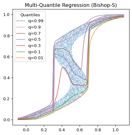
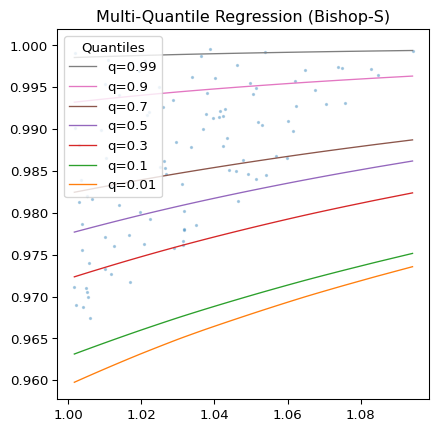
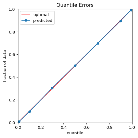
Picture 1 shows the results of a quantile regression using the deepquantiles Python package and the Bishop-S dataset.1 Picture 2 zooms into the upper right corner of the plot from Picture 1. Here the distribution is quite heteroskedastic, but the model successfully avoids quantile crossings. Picture 3 demonstrates that the quantiles, as predicted by the model, separate our random test sample as required.
Deep Learning for Quantile Regression
There are many ways to incorporate uncertainty into predictions. For instance, classical examples for modeling under uncertainty are time series models, such as ARIMA2 and GARCH3 or, more recently, NGBoost.4 But what if you want to use a different model that fits your problem, or perhaps a higher performing model? Deep Learning models can help with modeling under uncertainty in various ways. For instance, a separate deep learning model could learn to predict quantiles based on the predictions of an underlying model. Thereby, we could add quantiles to all kinds of interesting models that do not support this by default. As a first step, my colleague, Peter Prettenhofer, and I explored how well deep learning models predict the quantiles of various target distributions directly, not on top of the predictions of another model.
In the past, practitioners avoided deep learning models for uncertainty modeling. Deep learning models were hard to interpret, sensitive to hyperparameters, and required a lot of data and training time. Now, the transformer architecture5 is in the spotlight and powers successful tools like ChatGPT. A few years ago, the transformer architecture was mostly used to build large language models (LLMs). Now it is clear that it can be used with tabular data too.6
In our research, we adapted two existing solutions for our purposes to compare them with the quantiles we get from NGBoost’s predicted distributions using the percent point function:
- A custom multi-quantile regressor, DeepQuantiles, with an architecture that is similar to the multi-quantile regressor from the deepquantiles Python package. This is an example for a classical multi-layer neural network.
- The FTTransformer,7 which makes use of the transformer architecture like in state-of-the-art large language models but with a special tokenizer for numerical and categorical data.
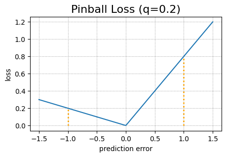
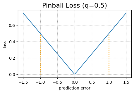
Both deep learning models use a tweaked pinball loss function to better cope with the problem of quantile crossings. The original pinball loss function is a standard loss function used for quantile regression. It consists of two parts. Let y be the true target value and ŷ the predicted target value. Then the pinball loss for a given quantile q is (1 – q)(ŷ – y) in case y < ŷ and q(y – ŷ) in case y ≥ ŷ.
Comparison
Below you see results for eight publicly available datasets often used for regression analysis with numerical and categorical variables and 506 to 11934 rows.
| ID | # Rows | # Categorical | # Numerical | # Values |
| ames-housing | 1,460 | 43 | 37 | 116,800 |
| concrete | 1,030 | 0 | 8 | 8,240 |
| energy | 768 | 0 | 8 | 6,144 |
| housing | 506 | 0 | 13 | 6,578 |
| kin8nm | 8,192 | 0 | 8 | 65,536 |
| naval | 11,934 | 0 | 16 | 190,944 |
| power | 9,568 | 0 | 4 | 38,272 |
| wine | 1599 | 0 | 11 | 17,589 |
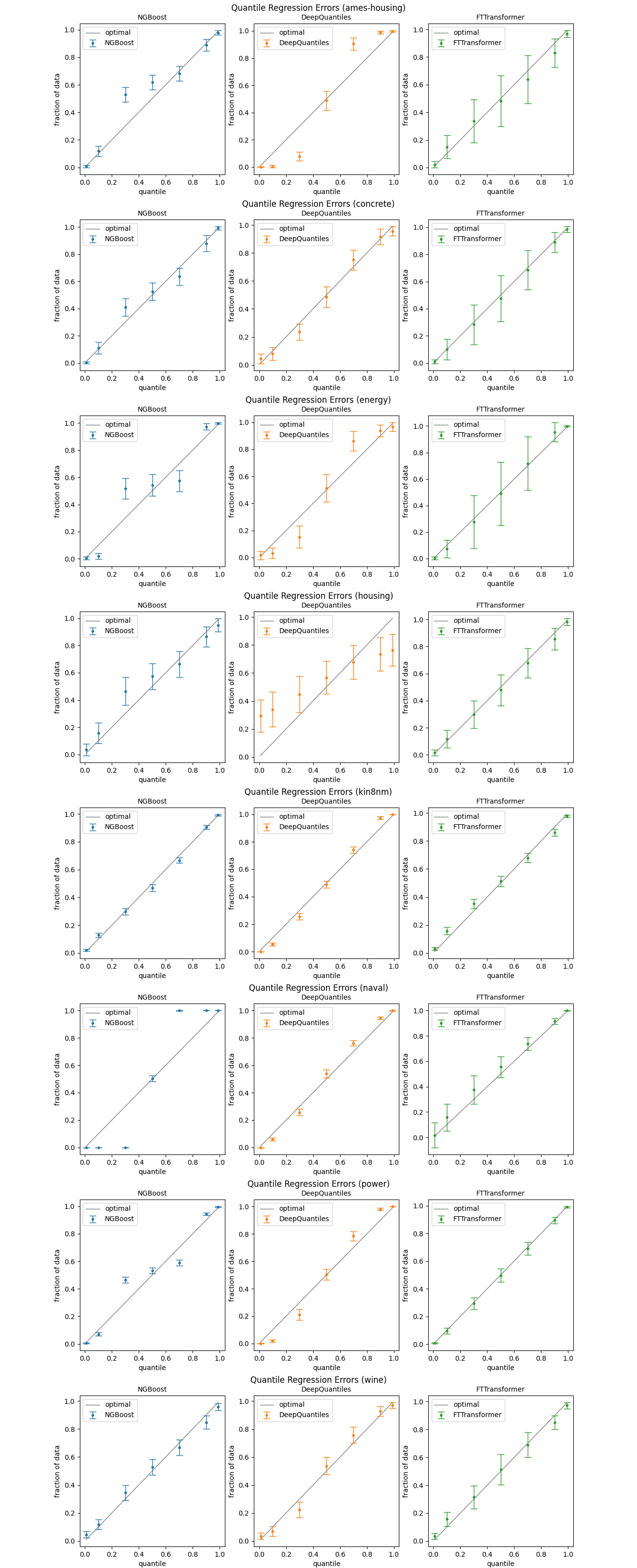
The plots below show the out-of-sample performance for the three models NGBoost, DeepQuantiles, and FTTransformer. We picked the quantiles 0.01, 0.1, 0.3, 0.5, 0.7, 0.9 and 0.99. For every model, we ran a 20-fold cross-validation with 5 repetitions. This means 100 runs per dataset. The dots depict the average predicted quantiles. The error bars are the standard deviations, not the standard errors.
Observations
NGBoost is doing a decent job but, apparently, has some problems with certain datasets (ames-housing, energy, naval, power). DeepQuantiles appears to be a bit stronger but also disappoints in a few cases (ames-housing, energy, housing). The FTTransformer gives very good results on average but with a huge variance.
One drawback of NGBoost is that it requires us to specify the type of distribution in advance. We did not make any additional assumptions and only used the default normal distribution. This could be the reason why NGBoost performs rather poorly on some datasets. Given that the performance of DeepQuantiles is quite sensitive to the choice of its hyperparameters, it is not a good alternative to NGBoost. In many situations, an ensemble of FTTransformers could be a good way to do quantile regression. The model is also not that sensitive to the choice of hyperparameters and is trained rather quickly.
Conclusion
We are constantly seeking to implement the learnings from our customers at DataRobot, and modeling under uncertainty is undoubtedly a very important capability that we are exploring. In this research, we saw that quantile regression is a simple way to do modeling under uncertainty and that the transformer architecture appears to be useful for that application. Deep learning even has the potential to enhance DataRobot regression models that currently lack this capability. Stay tuned, as we highlight even more innovations and research happening at DataRobot.
1 Pattern Recognition and Machine Learning, Christopher M. Bishop, Springer, 2007.
2 Time Series Analysis: Forecasting and Control, Jenkins, Gwilym M., et al. Wiley, 2015.
3 Generalized autoregressive conditional heteroskedasticity, Tim Bollerslev, Journal of Econometrics, vol. 31, no. 3, 1986, pp. 307-327.
4 arXiv, NGBoost: Natural Gradient Boosting for Probabilistic Prediction, Tony Duan, et al. 2019.
5 arXiv, Attention Is All You Need, Ashish Vaswani, et al. June 2017.
6 arXiv, Revisiting Deep Learning Models for Tabular Data, Yury Gorishniy, et al. June 2021.
7 Ibid
Related posts
See other posts in Inside the Product
Adopting agentic AI without addressing hallucinations is like ignoring a smoke detector. Learn how hallucinations reveal hidden risks across your AI workflows, and why they’re essential signals for building trustworthy, enterprise-ready agentic AI.

Eager to adopt agentic AI, but uncertain of the best path? The key is to move with intention, building on strong foundations at every step. Learn more about how to safely navigate the stages and avoid costly mistakes.

Deploy agentic AI faster with DataRobot and NVIDIA AI Enterprise. Learn how to rapidly develop and deliver agentic AI apps that solve complex use cases and transform work