Automating Model Risk Compliance: Model Monitoring

Monitoring Modern Machine Learning (ML) Methods In Production

In our previous two posts, we discussed extensively how modelers are able to both develop and validate machine learning models while following the guidelines outlined by the Federal Reserve Board (FRB) in SR 11-7. Once the model is successfully validated internally, the organization is able to productionize the model and use it to make business decisions. 

The question remains, however, once a model is productionized, how does the financial institution know if the model is still functioning for its intended purpose and design? Because models are a simplified representation of reality, many of the assumptions a modeler may have used when developing the model may not hold true when deployed live. If the assumptions are being breached due to fundamental changes in the process being modeled, the deployed system is not likely to serve its intended purpose, thereby creating further model risk that the institution must manage. The importance of managing this risk is highlighted further by the guidelines provided in SR 11-7:

Ongoing monitoring is essential to evaluate whether changes in products, exposures, activities, clients, or market conditions necessitate adjustment, redevelopment, or replacement of the model and to verify that any extension of the model beyond its original scope is valid.

Given the numerous variables that may change, how does the financial institution develop a robust monitoring strategy, and apply them in the context of ML models? In this post, we will discuss the considerations for ongoing monitoring as guided in SR 11-7, and show how DataRobot’s MLOps Platform enables organizations to make certain that their ML models are current and work for their intended purpose. 

Monitoring Model Metrics

Assumptions used in designing a machine learning model may be quickly violated due to changes in the process being modeled. This is often caused because the input data used to train the model was static and represented the world at one point in time, which is constantly changing. If these changes are not monitored, the decisions made from the model’s predictions may have a potentially deleterious impact. For example, we may have created a model to predict the demand for mortgage loans based upon macroeconomic data, including interest rates. If this model was trained over a period of time when interest rates were low, it may have the potential to overestimate the demand for such loans should interest rates or other macroeconomic variables change suddenly. Making resulting business decisions from this model may then be flawed, as the model has not captured the new reality and may need to be retrained. 

If we have constantly changing conditions that may render our model useless, how are we able to proactively identify them? A prerequisite in measuring a deployed model’s evolving performance is to collect both its input data and business outcomes in a deployed setting. With this data in hand, we are able to measure both the data drift and model performance, both of which are essential metrics in measuring the health of the deployed model. 

Mathematically speaking, data drift measures the shift in the distribution of input values used to train the model. In our mortgage demand example provided above, we may have had an input value that measured the average interest rate for different mortgage products. These observations would have spanned a distribution, which the model leveraged to make its forecasts. If, however, new policies by a central bank shifts the interest rates, we would correspondingly see a change in the distribution of values.

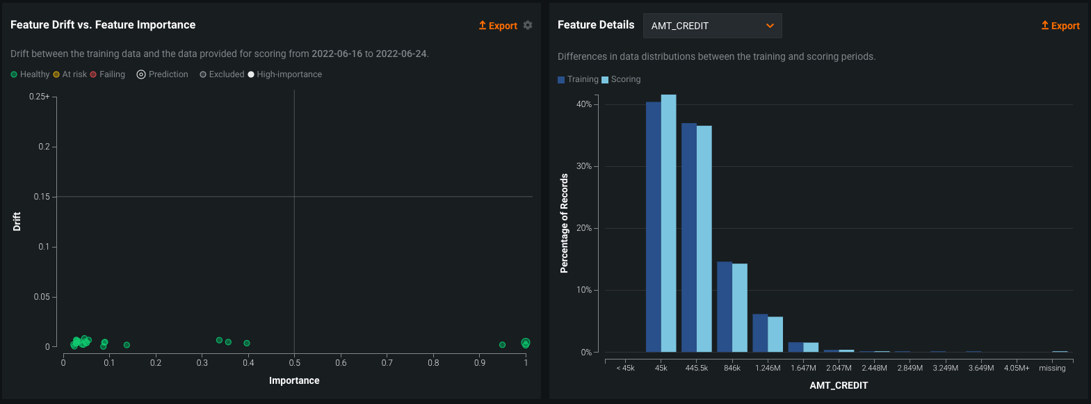
Within the data drift tab of a DataRobot deployment, users are able to both quantify the amount of shift that has occurred in the distribution, as well as visualize it. In the image below, we see two charts depicting the amount of drift that has occurred for a deployed model. 

On the left-hand side, we have a chart that depicts a scatter plot of the feature importance of a model input against drift. In this context, feature importance measures the importance of an input variable from a scale of 0 to 1, making use of the permutation importance metric when the model was trained. The closer this value is to 1, the more significant contribution it had on the model’s performance. On the y-axis of this same plot, we see drift is displayed – this is measured using a metric called population stability index, which quantifies the shift in the distribution of values between model training and in a production setting. On the right-hand side, we have a histogram that depicts the frequency of values for a particular input feature, comparing it between the data used to train the model (dark blue) and what was observed in a deployed setting (light blue). Combined with the Feature Drift plot on the left, these metrics are able to inform the modeler if there are any significant changes in the distribution of values in a live setting. 

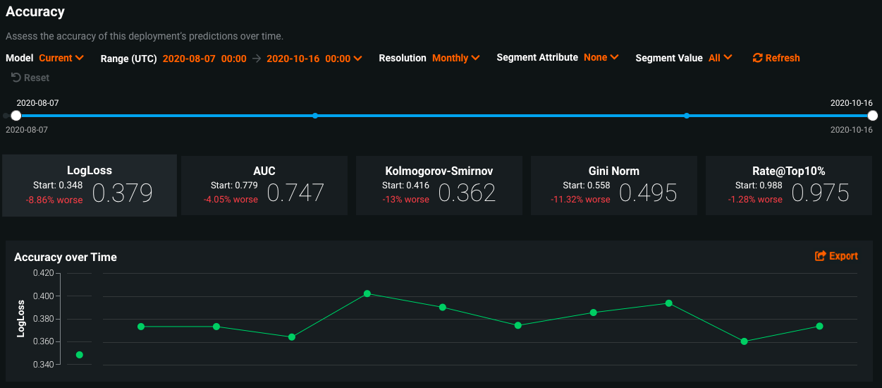
The accuracy of a model is another essential metric that informs us about its health in a deployed setting. Based upon the type of model deployed (classification vs. regression), there are a host of metrics we may use to quantify how accurate the prediction is. In the context of a classification model, we may have built a model that identifies whether or not a particular credit card transaction is fraudulent. In this context, as we deploy the model and make predictions against live data, we may observe if the actual outcome was indeed fraudulent. As we collect these business actuals, we may compute metrics that include the LogLoss of the model as well as its F1 score and AUC. 

Within DataRobot, the accuracy tab provides the owner of a model deployment with flexibility of what accuracy metrics they would like to monitor based upon their use case at hand. In the image below, we see an example of a deployed classification model that showcases a time series of how a model’s LogLoss metric has shifted over time, alongside a host of other performance metrics. 

Armed with a view of how data drift and accuracy has shifted in a production setting, the modeler is better equipped to understand if any of the assumptions used when training the model have been violated. Additionally, while observing actual business outcomes, the modeler is able to quantify decreases in accuracy, and decide whether or not to retrain the model based upon new data to ensure that it is still fit for its intended purpose. 

Model Benchmarking

Combined, telemetry on accuracy and data drift empowers the modeler to manage model risk for their organization, and thereby minimize the potential adverse impacts of a deployed ML model. While having such telemetry is crucial for sound model risk management principles, it is not, by itself, sufficient. Another fundamental principle of the modeling process as prescribed by SR 11-7 is the benchmarking of models placed into production with alternative models and theories. This is essential for managing model risk as it forces the modeler to revisit the original assumptions used to design the initial champion model, and try out a combination of different data inputs, model architectures, as well as target variables.

In DataRobot, modelers within the second line of defense are easily able to produce novel challenger models to provide an effective challenge against champion models produced by the first line of defense. The organization is then empowered to compare and contrast the performance of the challengers against the champion and see if it is appropriate to swap the challenger model with the champion, or keep the initial champion model as is. 

As a concrete example, a business unit with an organization may be tasked with developing credit risk scorecard models to determine the likelihood of default of a loan applicant. In the initial model design, the modeler may have, based upon their domain expertise, defined the target variable of default based upon whether or not the applicant repaid the loan within three months of being approved for the loan. When going through the validation process, another modeler in the second line of defense may have had good reason to redefine the target variable of default not based upon the window of three months, but rather six months. In addition, they may have also tried out combinations of different input features and model architectures that they believed had more predictive power. In the image shown below, they are able to register their model as a challenger to the deployed champion model within DataRobot and easily compare their performance. 

Overriding Model Predictions with Overlays

The importance of benchmarking in a sound MRM process can not be understated. The constant evaluation of key assumptions used to design a model are required to iterate on a model’s design, and ensure that it is serving its intended purpose. However, because models are only mathematical abstractions of reality, they are still subject to limitations, which the financial institution should acknowledge and account for. As stated in SR 11-7:

Ongoing monitoring should include the analysis of overrides with appropriate documentation. In the use of virtually any model, there will be cases where model output is ignored, altered, or reversed based on the expert judgment from model users. Such overrides are an indication that, in some respect, the model is not performing as intended or has limitations.

Within DataRobot, a modeler is empowered to set up override rules or model overlays on both the input data and model output. These Humility Rules within DataRobot acknowledge the limitations of models under certain conditions and enable the modeler to directly codify them and the override action to take. For example, if we had built a model to identify fraudulent credit card transactions, it may have been the case that we only observed samples from a particular geographic region, like North America. In a production setting, however, we may observe transactions that had occurred in other countries, which we either had very few samples for, and or were not present at all in the training data. Under such circumstances, our model may not be able to make reliable predictions for a new geography, and we would rather apply a default rule or send that transaction to a risk analyst. With Humility Rules, the modeler is able to codify trigger rules and apply the appropriate override. This has the impact of making sure the institution is able to use expert judgment in cases where the model is not reliable, thereby minimizing model risk.

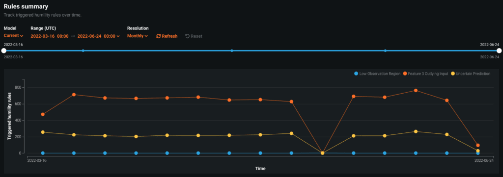
The image below showcases an example of a model deployment which has different Humility Rules that have been applied. In addition to providing rules for values that were not seen frequently while training a model, a modeler is able to also set up rules based upon how certain the model output is, as well as rules for treating feature values that are outliers.

When humility rules and triggers have been set in place, a modeler is able to monitor the number of times they have been invoked. Revisiting our fraudulent transaction example described above, if we do observe that in a production setting we have many samples from Europe, it may be reason to revisit the assumptions used in the initial model design and potentially retrain the model on a wider geographic area to make sure it is still functioning reliably. As shown below, the modeler is able to look at the time series visualization as shown below to determine if a rule has been triggered at an alarming rate during the life of a deployed model.

Conclusion

Ongoing model monitoring is an essential component of a sound model risk management practice. Because models only capture the state of the world at a specific point in time, the performance of a deployed model may dramatically deteriorate due to changing outside conditions. To ensure that models are working for their intended purpose, a key prerequisite is to collect model telemetry data in a production setting, and use it to measure health metrics that include data drift and accuracy. By understanding the evolving performance of the model and revisiting the assumptions used to initially design it, the modeler may develop challenger models to help ensure that the model is still performant and fit for its intended business purpose. Lastly, due to the limitations of any model, the modeler is able to set up rules to make sure that expert judgment overrides a model output in uncertain/extreme circumstances. By incorporating these strategies within the lifecycle of a model, the organization is able to minimize the potential adverse impact that a model may have on the business.

About the author

Harsh Patel

Data Platform Architect - Field CTO Office, Snowflake

Harsh Patel is a Customer-Facing Data Scientist at DataRobot. He leverages the DataRobot platform to drive the adoption of AI and Machine Learning at major enterprises in the United States, with a specific focus within the Financial Services Industry. Prior to DataRobot, Harsh worked in a variety of data-centric roles in both startups and major enterprises, where he had the opportunity to build many data products leveraging machine learning.
Harsh studied Physics and Engineering at Cornell University, and in his spare time enjoys traveling and exploring the parks in NYC.

Meet Harsh Patel